Hands-on Exercise 4 - Visual Statistical Analysis

Author

Alicia Loh

Published

April 27, 2024

Modified

May 1, 2024

Learning Objectives:

Create visual graphics with rich statistical information using ggstatsplot package
Use performance package to visualise model diagnostics
Use parameters package to visualise model parameters

Getting Started

ggstatsplot is an extension of ggplot2 package for creating graphics with details from statistical tests included in the information-rich plots themselves.

To provide alternative statistical inference methods by default
To follow besst practices for statistical reporting
For all statistical tests resulted in the plots, the default template abides by the APA gold standard for statistical reporting

Installing and loading the required libraries

The following R packages will be used:

ggstatsplotis an extension of ggplot2 package for creating graphics with details from statstical tests included in the plots themselces
tidyverse, a family of modern R packages specially designed to support data science, analysis and communication task including creating static statistical graphs.

Code chunk below will be used to check if these packages have been installed and also will load them into the working R environment.

pacman::p_load(ggstatsplot, tidyverse)

Importing the Data

The code chunk below imports exam_data.csv into R environment by using read_csv() function of readr package.
readr is a pacakge within tidyverse.

exam <- read_csv("data/Exam_data.csv")

exam_data tibble data frame contains:

Year end examination grades of a cohort of primary 3 students from a local school.
There are a total of seven attributes. Four of them are categorical data type and the other three are in continuous data type.
- The categorical attributes are: ID, CLASS, GENDER and RACE.
- The continuous attributes are: MATHS, ENGLISH and SCIENCE.

**One-sample test: gghistostats() method**

In the code chunk below, gghistostats() is used to to build an visual of one-sample test on English scores.

Plot
Code

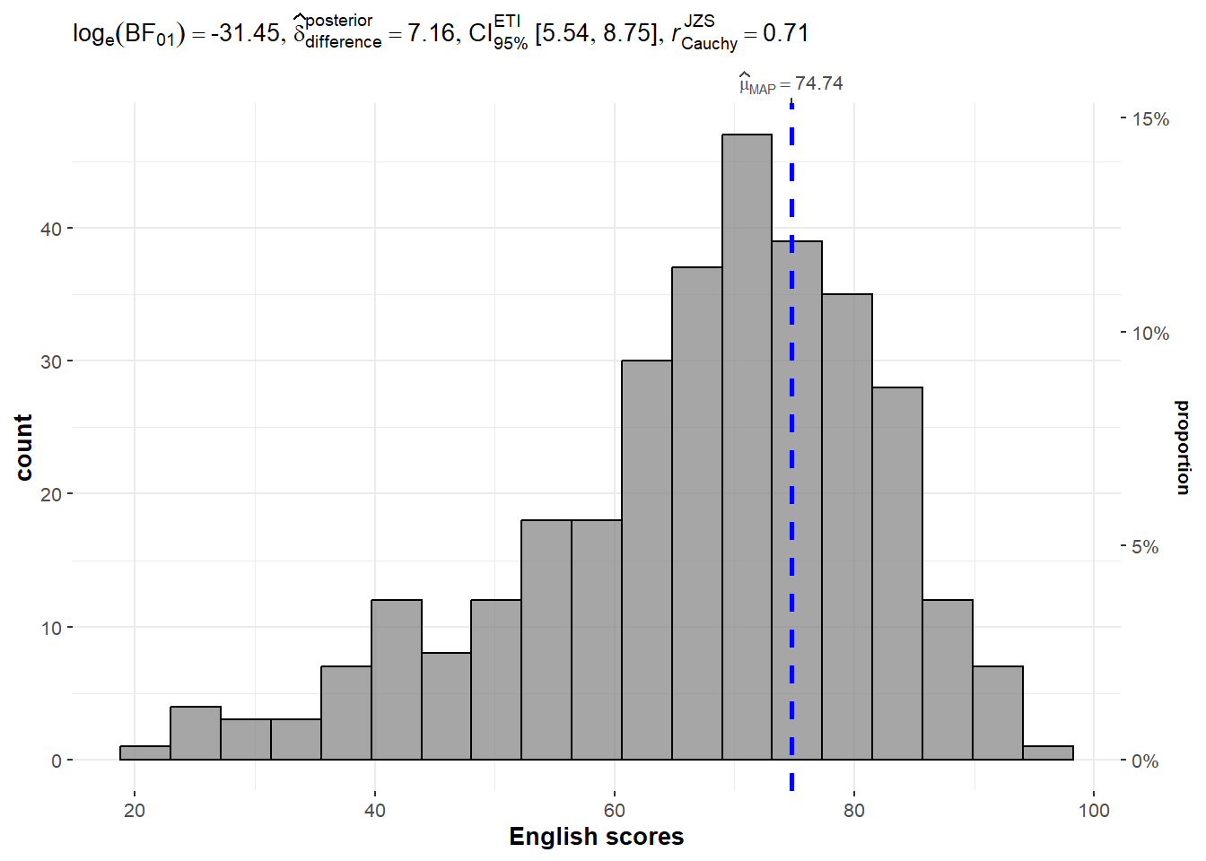
set.seed(1234) # for reproducibility

gghistostats(
  data = exam,
  x = ENGLISH,
  type = "bayes",
  test.value = 60,
  xlab = "English scores"
)

Default information: - statistical details - Bayes Factor - sample sizes - distribution summary

Unpacking the Bayes Factor

A Bayes factor is the ratio of the likelihood of one particular hypothesis to the likelihood of another. i.e., a measure of the strength of evidence in favor of one theory among two competing theories.
Bayes factor allows evaluation of the data in favor of a null hypothesis, and to use external information to do so. It gives the weight of the evidence in favor of a given hypothesis.
When comparing two hypotheses, H₁ (the alternate hypothesis) and H₀ (the null hypothesis), the Bayes Factor is often written as B₁₀, defined mathematically as:

$\frac{l i k e l i h o o d o f d a t a g i v e n H_{1}}{l i k e l i h o o d o f d a t a g i v e n H_{0}} = \frac{P (D | H_{1})}{P (D | H_{0})}$
The Schwarz criterion is one of the easiest ways to calculate rough approximation of the Bayes Factor.

Interpreting Bayes Factor

A Bayes Factor can be any positive number. A common interpretation was first proposed by Harold Jeffereys (1961) and slightly modified by Lee and Wagenmakers in 2013:

B10 Value	Conclusion
>100	Extreme evidence for H₁
30-100	Very strong evidence for H₁
10-30	Strong evidence for H₁
3-10	Moderate evidence for H₁
1-3	Anecdotal evidence for H₁
1	No evidence
1/3-1	Anecdotal evidence for H₁
1/3-1/10	Moderate evidence for H₁
1/10-1/30	Strong evidence for H₁
1/30-1/100	Very strong evidence for H₁
<1/100	Extreme evidence for H₁

Two-sample mean test: ggbetweenstats()

In the code chunk below, ggbetweenstats() is used to build a visual for two-sample mean test of Maths scores by gender.

Plot
Code

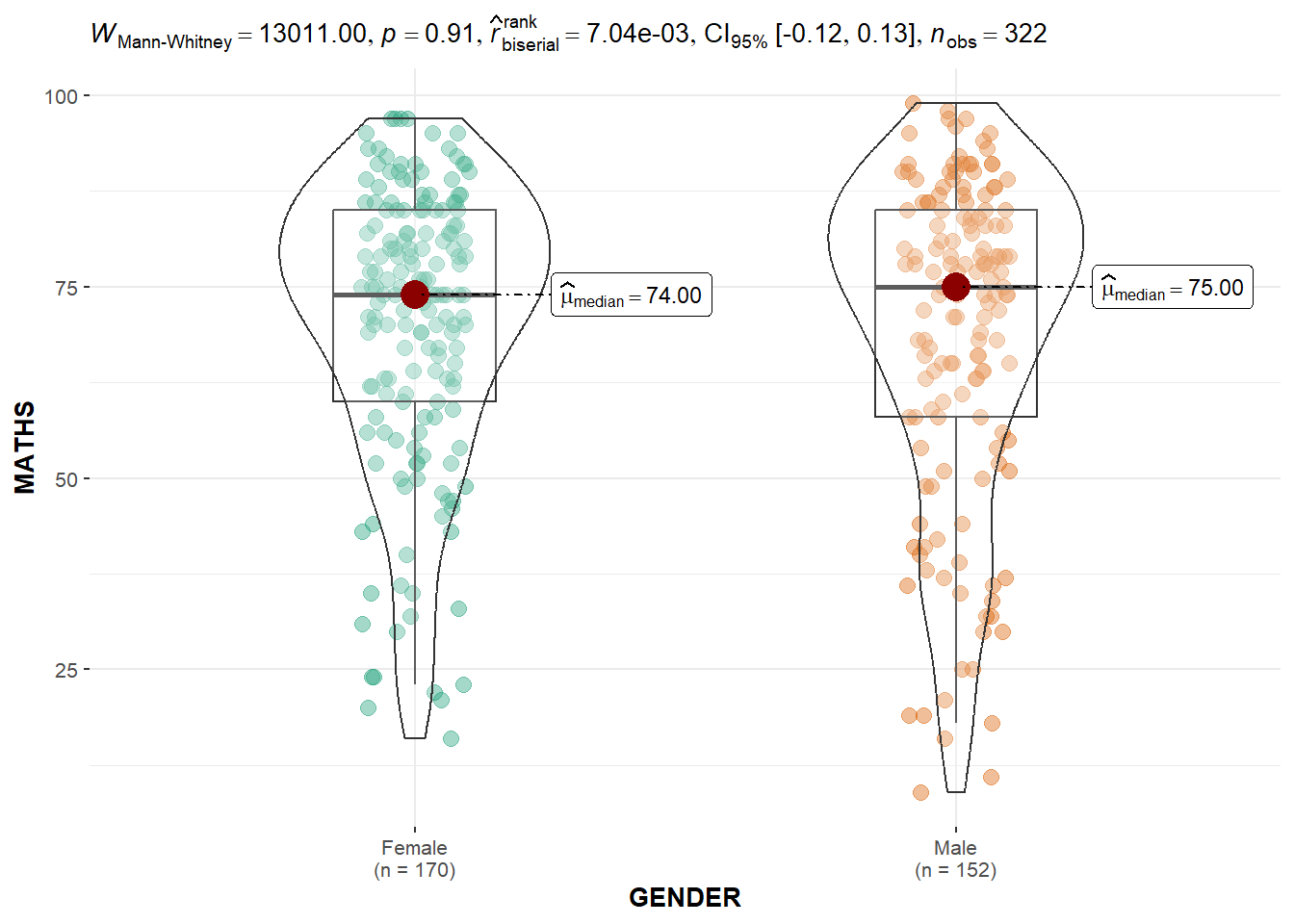
ggbetweenstats(
  data = exam,
  x = GENDER, 
  y = MATHS,
  type = "np",
  messages = FALSE
)

Default information: - statistical details - Bayes Factor - sample sizes - distribution summary

**Oneway ANOVA Test: ggbetweenstats() method**

In the code chunk below, ggbetweenstats() is used to build a visual for One-way ANOVA test on English score by race.

Plot
Code

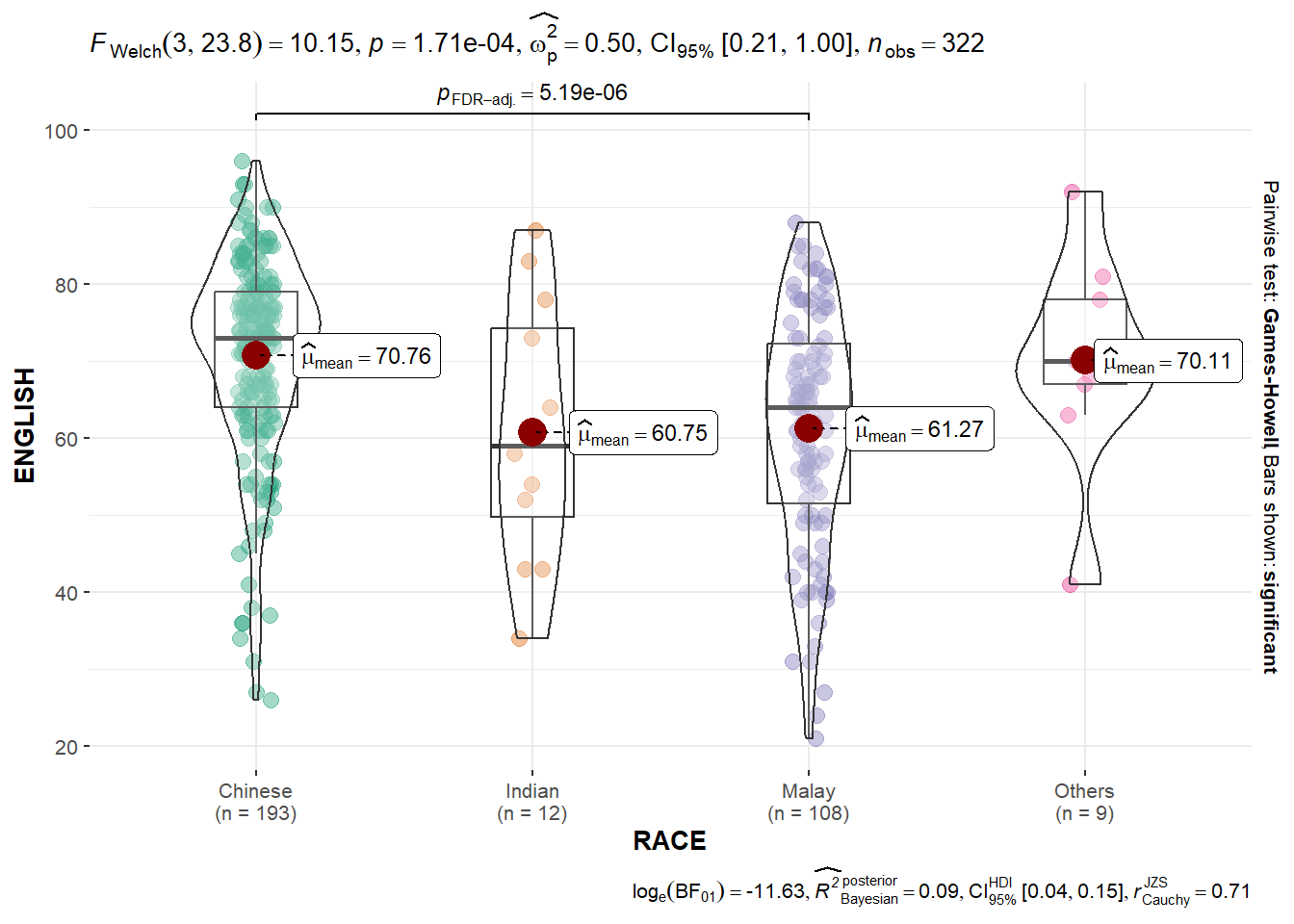
ggbetweenstats(
  data = exam,
  x = RACE, 
  y = ENGLISH,
  type = "p",
  mean.ci = TRUE, 
  pairwise.comparisons = TRUE, 
  pairwise.display = "s",
  p.adjust.method = "fdr",
  messages = FALSE
)

“ns” → only non-significant
“s” → only significant
“all” → everything

ggbetweenstats - Summary of tests

Following (between-subjects) tests are carried out for each type of analyses:

Type	No. of groups	Test
Parametric	>2	Fisher’s or Welch’s one-way ANOVA
Non-parametric	>2	Kruskal-Wallis one-way ANOVA
Robust	>2	Heteroscedastic one-way ANOVA for trimmed means
Bayes Factor	>2	Fisher’s ANOVA
Parametric	2	Student’s or Welch’s t-test
Non-parametric	2	Mann-Whitney U test
Robust	2	Yuen’s test for trimmed means
Bayes Factor	2	Student’s t-test

Following effect sizes (and confidence intervals) are available for each type of test:

Type	No. of Groups	Effect Size	Confidence Intervals
Parametric	>2	${η^{2}}_{p}, η^{2}, {ω^{2}}_{p}, ω^{2}$	Yes
Non-parametric	>2	${η^{2}}_{H}$ (H-statistic based eta-squared)	Yes
Robust	>2	$ξ$ (Explanatory measure of effect size)	Yes
Bayes Factor	>2	No	No
Parametric	2	Cohen’s d, Hedge’s g (central-and-noncentral-t distribution based)	Yes
Non-parametric	2	r (computed as $Z / \sqrt{N}$ )	Yes
Robust	2	$ξ$ (Explanatory measure of effect size)	Yes
Bayes Factor	2	No	No

Summary of pairwise comparison tests supported in ggbetweenstats

Type	Equal Variance	Test	p-value Adjustment?
Parametric	No	Games Howell Test	Yes
Parametric	Yes	Student’s t Test	Yes
Non-Parametric	No	Dunn Test	Yes
Robust	No	Yuen’s Trimmed Means Test	Yes
Bayes Factor	NA	Student’s t Test	NA

Significant Test of Correlation: ggscatterstats()

In the code chunk below, ggscatterstats() is used to build a visual for Significant Test of Correlation between Maths scores and English scores.

Plot
Code

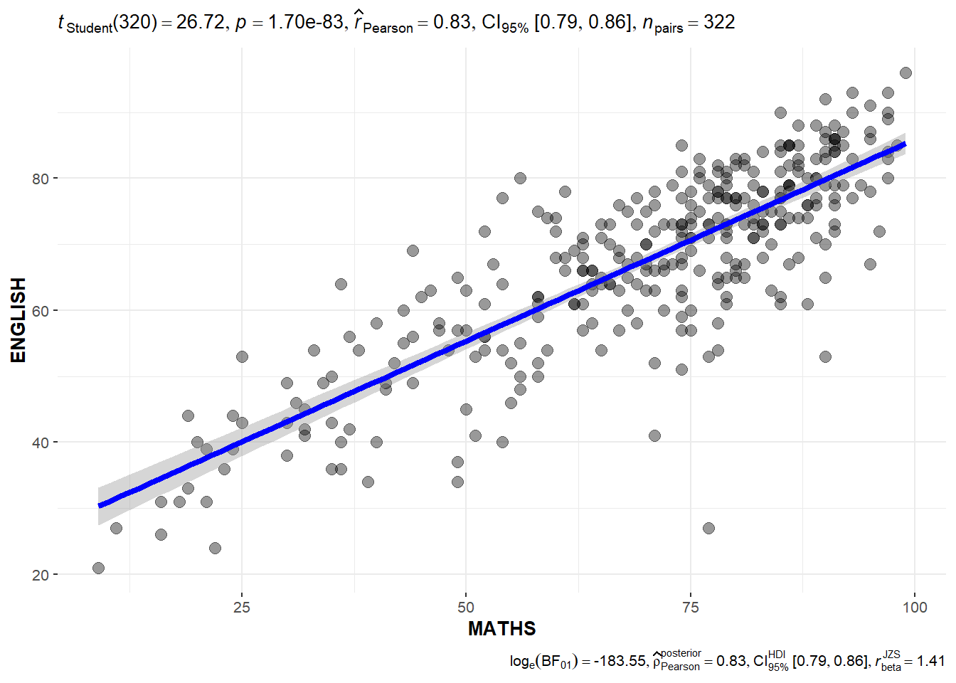
ggscatterstats(
  data = exam,
  x = MATHS,
  y = ENGLISH,
  marginal = FALSE,
  )

**Significant Test of Association (Depedence) : ggbarstats() methods**

In the code chunk below, the Maths scores is binned into a 4-class variable by using cut(). ggbarstats() is used to build a visual for Significant Test of Association

Plot
Code

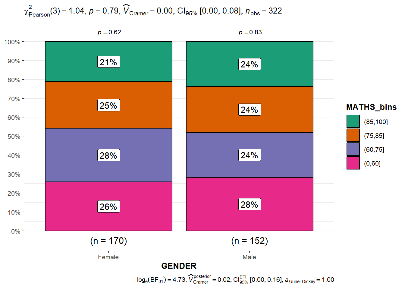
exam1 <- exam %>% 
  mutate(MATHS_bins = 
           cut(MATHS, 
               breaks = c(0,60,75,85,100))
)

ggbarstats(exam1, 
           x = MATHS_bins, 
           y = GENDER)

Visualising Models

Visualise model diagnostic and model parameters by using parameters package.

Toyota Corolla case study will be used. The purpose of study is to build a model to discover factors affecting prices of used-cars by taking into consideration a set of explanatory variables.

Installing and loading the required libraries

pacman::p_load(readxl, performance, parameters, see)

Importing Excel file: readxl methods

In the code chunk below, read_xls() of readxl package is used to import the data worksheet of ToyotaCorolla.xls workbook into R.

car_resale <- read_xls("data/ToyotaCorolla.xls", 
                       "data")
car_resale

# A tibble: 1,436 × 38
      Id Model    Price Age_08_04 Mfg_Month Mfg_Year     KM Quarterly_Tax Weight
   <dbl> <chr>    <dbl>     <dbl>     <dbl>    <dbl>  <dbl>         <dbl>  <dbl>
 1    81 TOYOTA … 18950        25         8     2002  20019           100   1180
 2     1 TOYOTA … 13500        23        10     2002  46986           210   1165
 3     2 TOYOTA … 13750        23        10     2002  72937           210   1165
 4     3  TOYOTA… 13950        24         9     2002  41711           210   1165
 5     4 TOYOTA … 14950        26         7     2002  48000           210   1165
 6     5 TOYOTA … 13750        30         3     2002  38500           210   1170
 7     6 TOYOTA … 12950        32         1     2002  61000           210   1170
 8     7  TOYOTA… 16900        27         6     2002  94612           210   1245
 9     8 TOYOTA … 18600        30         3     2002  75889           210   1245
10    44 TOYOTA … 16950        27         6     2002 110404           234   1255
# ℹ 1,426 more rows
# ℹ 29 more variables: Guarantee_Period <dbl>, HP_Bin <chr>, CC_bin <chr>,
#   Doors <dbl>, Gears <dbl>, Cylinders <dbl>, Fuel_Type <chr>, Color <chr>,
#   Met_Color <dbl>, Automatic <dbl>, Mfr_Guarantee <dbl>,
#   BOVAG_Guarantee <dbl>, ABS <dbl>, Airbag_1 <dbl>, Airbag_2 <dbl>,
#   Airco <dbl>, Automatic_airco <dbl>, Boardcomputer <dbl>, CD_Player <dbl>,
#   Central_Lock <dbl>, Powered_Windows <dbl>, Power_Steering <dbl>, …

Multiple Regression Model using lm()

The code chunk below is used to calibrate a multiple linear regression model by using lm() of Base Stats of R.

model <- lm(Price ~ Age_08_04 + Mfg_Year + KM + 
              Weight + Guarantee_Period, data = car_resale)
model


Call:
lm(formula = Price ~ Age_08_04 + Mfg_Year + KM + Weight + Guarantee_Period, 
    data = car_resale)

Coefficients:
     (Intercept)         Age_08_04          Mfg_Year                KM  
      -2.637e+06        -1.409e+01         1.315e+03        -2.323e-02  
          Weight  Guarantee_Period  
       1.903e+01         2.770e+01

Model Diagnostic: checking for multicolinearity:

In the code chunk, check_collinearity() of performance package.

check_collinearity(model)

# Check for Multicollinearity

Low Correlation

             Term  VIF     VIF 95% CI Increased SE Tolerance Tolerance 95% CI
               KM 1.46 [ 1.37,  1.57]         1.21      0.68     [0.64, 0.73]
           Weight 1.41 [ 1.32,  1.51]         1.19      0.71     [0.66, 0.76]
 Guarantee_Period 1.04 [ 1.01,  1.17]         1.02      0.97     [0.86, 0.99]

High Correlation

      Term   VIF     VIF 95% CI Increased SE Tolerance Tolerance 95% CI
 Age_08_04 31.07 [28.08, 34.38]         5.57      0.03     [0.03, 0.04]
  Mfg_Year 31.16 [28.16, 34.48]         5.58      0.03     [0.03, 0.04]

check_c <- check_collinearity(model)
plot(check_c)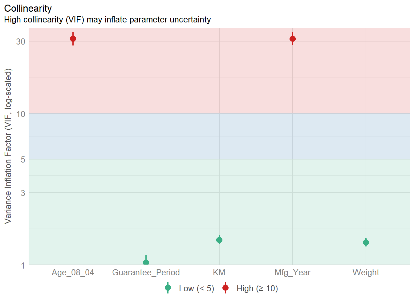

Model Diagnostic: checking normality assumption

In the code chunk, check_normality() of performance package.

Plot
Code

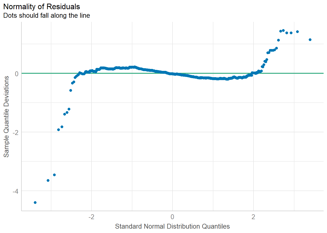
model1 <- lm(Price ~ Age_08_04 + KM + 
              Weight + Guarantee_Period, data = car_resale)

check_n <- check_normality(model1)

plot(check_n)

Model Diagnostic: Check model for homogeneity of variances

In the code chunk, check_heteroscedasticity() of performance package.

Plot
Code

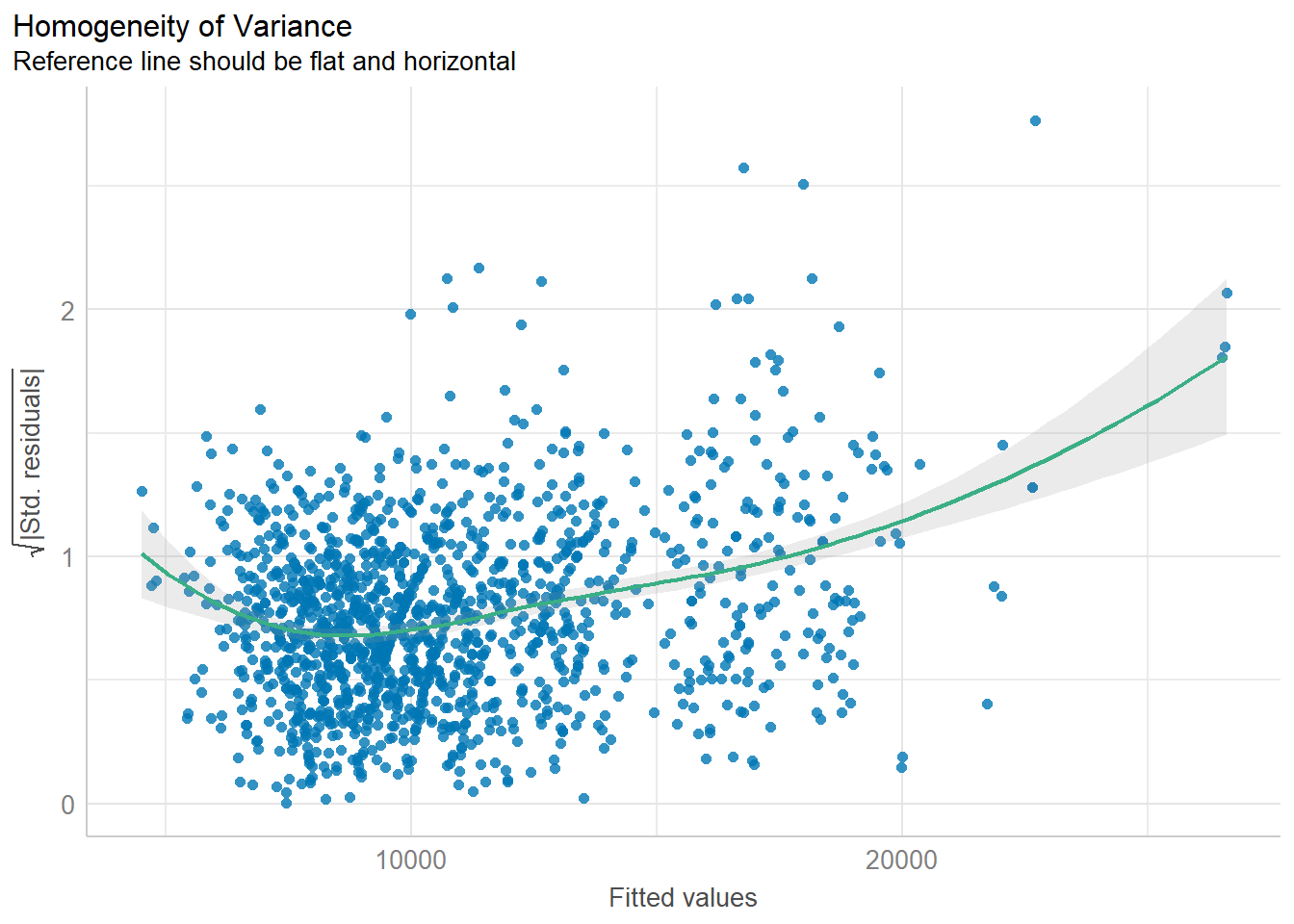
check_h <- check_heteroscedasticity(model1)
plot(check_h)

Model Diagnostic: Complete check

We can also perform the complete by using check_model().

Plot
Code

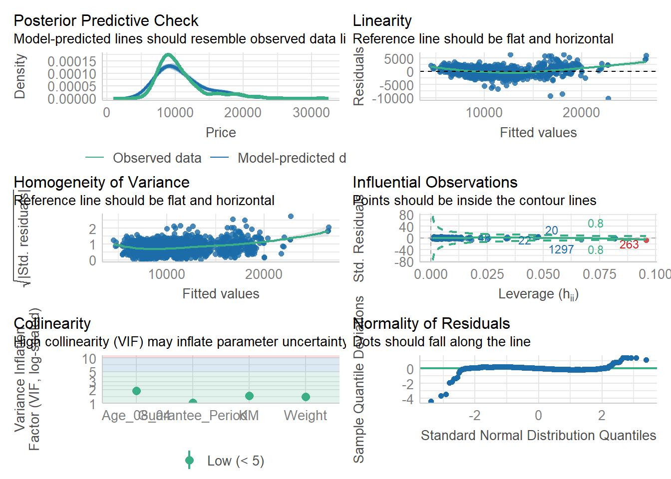
check_model(model1)

Visualising Regression Parameters: see methods

In the code below, plot() of see package and parameters() of parameters package is used to visualise the parameters of a regression model.

Plot
Code

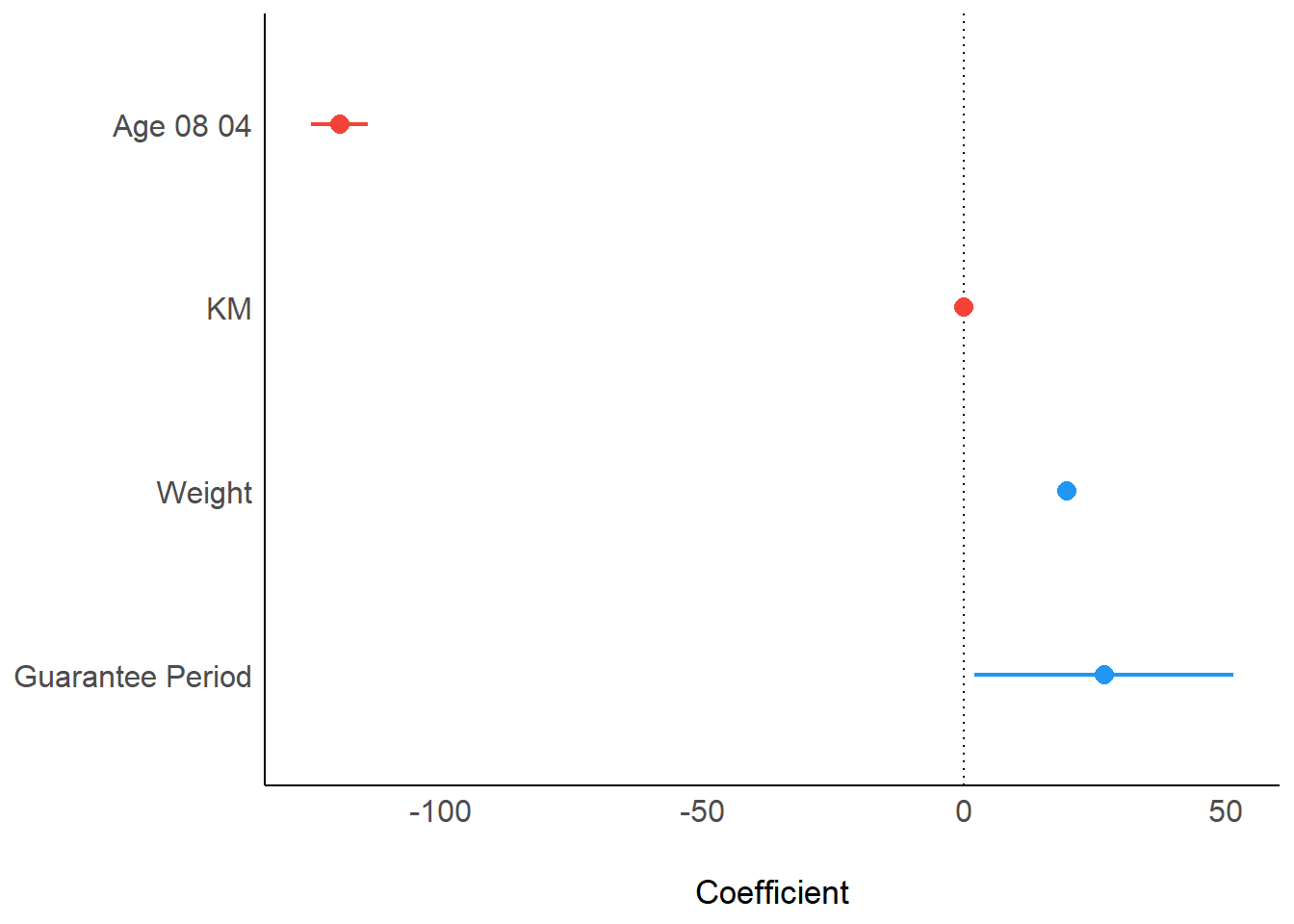
plot(parameters(model1))

**Visualising Regression Parameters: ggcoefstats() methods**

In the code below, ggcoefstats() of ggstatsplot package to visualise the parameters of a regression model.

Plot
Code

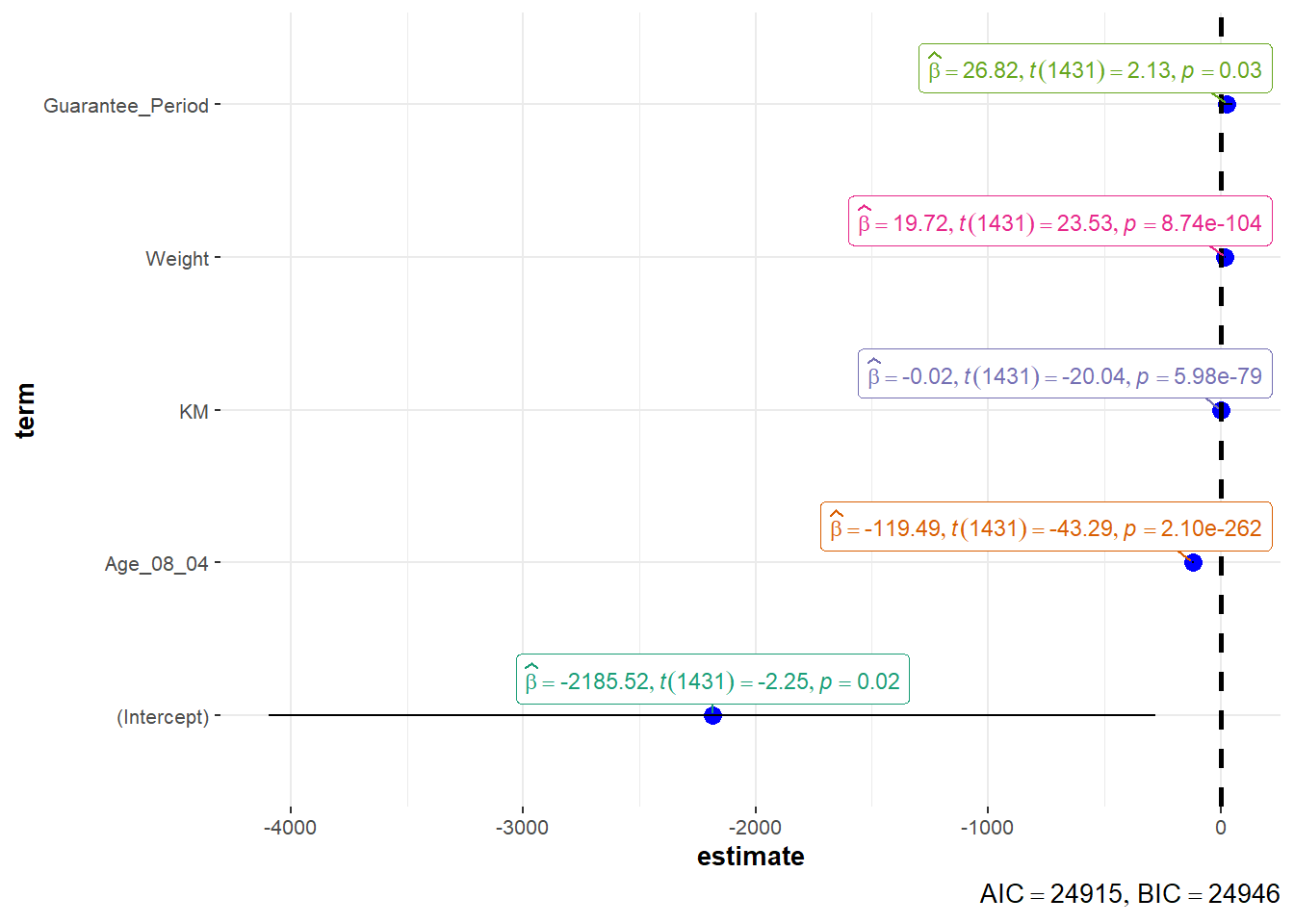
ggcoefstats(model1, 
            output = "plot")