pacman::p_load(tidyverse)Take-home Exercise 1 - Creating Data Visualisation Beyond Default (Geographical Distribution)
Geographical Distribution
Take-home Exercise 1 focuses on statistical graphic methods for visualising frequency distribution and value distribution using ggplot2 and its extensions. The below section is an exploration of the data’s geographical distribution on my own accord.
Downloading the Dataset

To accomplish the task, transaction data of REALIS will be used.
Access Dataset via SMU e-library
After logging in with SMU credentials, navigate to “Residential” tab
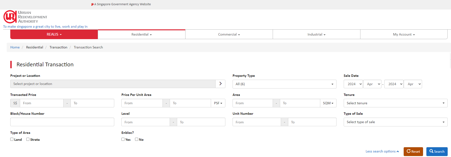
Under Property Types, “Select All”
Under Sale Date, select “2024 Jan” - “2024 Mar”
Click “Search”
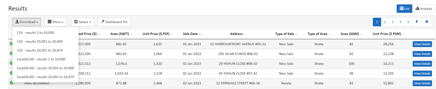
Click “Download”
Due to the size of the dataset, it is split into multiple segments. Download all in .csv format
The Designing Tool
The data will be processed using the appropriate tidyverse family of packages and the statistical graphics will be prepared using ggplot2 and its extensions.
Getting Started
Installing and loading the required libraries
Note: Ensure that the pacman package has already been installed.
The code chunk below loads the following packages using uses p_load() of pacman package:
- tidyverse: (i.e. readr, tidyr, dplyr, ggplot2, lubridate) for performing data science tasks such as importing, tidying, and wrangling data, as well as creating graphics based on The Grammar of Graphics
Importing the Data
The data has been split into multiple .csv files
list.files()list all CSV files in the specified directory.After looping through each CSV file, read it into a data frame using
read_csv(), and store it in a list.bind_rows()combines all data frames in the list into a single big data frame.
csv_directory <- "data/"
csv_files <- list.files(csv_directory, pattern = "\\.csv$", full.names = TRUE)
realis <- list()
for (file in csv_files) {
realis[[file]] <- read_csv(file)
}realis_all <- bind_rows(realis)View Data
names()function prints the names of the columns in the tibble data frame.glimpse()function gives a quick overview of the tibble data frame
col_names <- names(realis_all)
col_names [1] "Project Name" "Transacted Price ($)"
[3] "Area (SQFT)" "Unit Price ($ PSF)"
[5] "Sale Date" "Address"
[7] "Type of Sale" "Type of Area"
[9] "Area (SQM)" "Unit Price ($ PSM)"
[11] "Nett Price($)" "Property Type"
[13] "Number of Units" "Tenure"
[15] "Completion Date" "Purchaser Address Indicator"
[17] "Postal Code" "Postal District"
[19] "Postal Sector" "Planning Region"
[21] "Planning Area" glimpse(realis_all)Rows: 26,806
Columns: 21
$ `Project Name` <chr> "THE REEF AT KING'S DOCK", "URBAN TREASU…
$ `Transacted Price ($)` <dbl> 2317000, 1823500, 1421112, 1258112, 1280…
$ `Area (SQFT)` <dbl> 882.65, 882.65, 1076.40, 1033.34, 871.88…
$ `Unit Price ($ PSF)` <dbl> 2625, 2066, 1320, 1218, 1468, 1767, 1095…
$ `Sale Date` <chr> "01 Jan 2023", "02 Jan 2023", "02 Jan 20…
$ Address <chr> "12 HARBOURFRONT AVENUE #05-32", "205 JA…
$ `Type of Sale` <chr> "New Sale", "New Sale", "New Sale", "New…
$ `Type of Area` <chr> "Strata", "Strata", "Strata", "Strata", …
$ `Area (SQM)` <dbl> 82.0, 82.0, 100.0, 96.0, 81.0, 308.7, 42…
$ `Unit Price ($ PSM)` <dbl> 28256, 22238, 14211, 13105, 15802, 19015…
$ `Nett Price($)` <chr> "-", "-", "-", "-", "-", "-", "-", "-", …
$ `Property Type` <chr> "Condominium", "Condominium", "Executive…
$ `Number of Units` <dbl> 1, 1, 1, 1, 1, 1, 1, 1, 1, 1, 1, 1, 1, 1…
$ Tenure <chr> "99 yrs from 12/01/2021", "Freehold", "9…
$ `Completion Date` <chr> "Uncompleted", "Uncompleted", "Uncomplet…
$ `Purchaser Address Indicator` <chr> "HDB", "Private", "HDB", "HDB", "HDB", "…
$ `Postal Code` <chr> "097996", "419535", "269343", "269294", …
$ `Postal District` <chr> "04", "14", "27", "27", "28", "19", "10"…
$ `Postal Sector` <chr> "09", "41", "26", "26", "79", "54", "27"…
$ `Planning Region` <chr> "Central Region", "East Region", "North …
$ `Planning Area` <chr> "Bukit Merah", "Bedok", "Yishun", "Yishu…
Note
realis_all contains:
Public and Private residential property transaction data from 1st January 2023 to 31st March 2024.
There are 26,806 rows and 21 columns.
Data Preparation
Standardise Date Format
The “Sales Date” column is currently a cha type. It needs to be converted into date format.
dmy() is a function from the lubridate package that converts character strings to date format in the day-month-year (DMY) order.
realis_all$`Sale Date` <- dmy(realis_all$`Sale Date`)head(realis_all$`Sale Date`)[1] "2023-01-01" "2023-01-02" "2023-01-02" "2023-01-02" "2023-01-03"
[6] "2023-01-03"Keep Relevant Rows
Duplicate and empty rows are removed.
qa_pte_raw <- realis_all %>%
distinct() %>%
drop_na()View Data
glimpse(qa_pte_raw)Rows: 26,800
Columns: 21
$ `Project Name` <chr> "THE REEF AT KING'S DOCK", "URBAN TREASU…
$ `Transacted Price ($)` <dbl> 2317000, 1823500, 1421112, 1258112, 1280…
$ `Area (SQFT)` <dbl> 882.65, 882.65, 1076.40, 1033.34, 871.88…
$ `Unit Price ($ PSF)` <dbl> 2625, 2066, 1320, 1218, 1468, 1767, 1095…
$ `Sale Date` <date> 2023-01-01, 2023-01-02, 2023-01-02, 202…
$ Address <chr> "12 HARBOURFRONT AVENUE #05-32", "205 JA…
$ `Type of Sale` <chr> "New Sale", "New Sale", "New Sale", "New…
$ `Type of Area` <chr> "Strata", "Strata", "Strata", "Strata", …
$ `Area (SQM)` <dbl> 82.0, 82.0, 100.0, 96.0, 81.0, 308.7, 42…
$ `Unit Price ($ PSM)` <dbl> 28256, 22238, 14211, 13105, 15802, 19015…
$ `Nett Price($)` <chr> "-", "-", "-", "-", "-", "-", "-", "-", …
$ `Property Type` <chr> "Condominium", "Condominium", "Executive…
$ `Number of Units` <dbl> 1, 1, 1, 1, 1, 1, 1, 1, 1, 1, 1, 1, 1, 1…
$ Tenure <chr> "99 yrs from 12/01/2021", "Freehold", "9…
$ `Completion Date` <chr> "Uncompleted", "Uncompleted", "Uncomplet…
$ `Purchaser Address Indicator` <chr> "HDB", "Private", "HDB", "HDB", "HDB", "…
$ `Postal Code` <chr> "097996", "419535", "269343", "269294", …
$ `Postal District` <chr> "04", "14", "27", "27", "28", "19", "10"…
$ `Postal Sector` <chr> "09", "41", "26", "26", "79", "54", "27"…
$ `Planning Region` <chr> "Central Region", "East Region", "North …
$ `Planning Area` <chr> "Bukit Merah", "Bedok", "Yishun", "Yishu…
Note
qa_pte_raw contains:
Private residential property transaction data from 1st January 2023 to 31st March 2024
There are 26,800 rows and 21 columns.
Keep Relevant Columns
Not all 21 columns will be used for analysis e.g. contains overlapping information as another column. Only relevant columns will be kept.
Columns to drop:
Area (SQFT): Similar information as Area (SQM)
Unit Price ($ PSF): Similar information as Unit Price ($ PSM)
Nett Price ($): Similar information as Transacted Price ($)
Postal District and Postal Sector: Overlapping information as Postal Code
Columns to be dropped can be specified by prefixing the column names with a minus sign (-) when using the select() function from the dplyr package.
qa_pte <- qa_pte_raw %>%
select(
-`Area (SQFT)`,
-`Unit Price ($ PSF)`,
-`Postal District`,
-`Postal Sector`
)glimpse(qa_pte)Rows: 26,800
Columns: 17
$ `Project Name` <chr> "THE REEF AT KING'S DOCK", "URBAN TREASU…
$ `Transacted Price ($)` <dbl> 2317000, 1823500, 1421112, 1258112, 1280…
$ `Sale Date` <date> 2023-01-01, 2023-01-02, 2023-01-02, 202…
$ Address <chr> "12 HARBOURFRONT AVENUE #05-32", "205 JA…
$ `Type of Sale` <chr> "New Sale", "New Sale", "New Sale", "New…
$ `Type of Area` <chr> "Strata", "Strata", "Strata", "Strata", …
$ `Area (SQM)` <dbl> 82.0, 82.0, 100.0, 96.0, 81.0, 308.7, 42…
$ `Unit Price ($ PSM)` <dbl> 28256, 22238, 14211, 13105, 15802, 19015…
$ `Nett Price($)` <chr> "-", "-", "-", "-", "-", "-", "-", "-", …
$ `Property Type` <chr> "Condominium", "Condominium", "Executive…
$ `Number of Units` <dbl> 1, 1, 1, 1, 1, 1, 1, 1, 1, 1, 1, 1, 1, 1…
$ Tenure <chr> "99 yrs from 12/01/2021", "Freehold", "9…
$ `Completion Date` <chr> "Uncompleted", "Uncompleted", "Uncomplet…
$ `Purchaser Address Indicator` <chr> "HDB", "Private", "HDB", "HDB", "HDB", "…
$ `Postal Code` <chr> "097996", "419535", "269343", "269294", …
$ `Planning Region` <chr> "Central Region", "East Region", "North …
$ `Planning Area` <chr> "Bukit Merah", "Bedok", "Yishun", "Yishu…
Note
qa_pte contains:
Private residential property transaction data from 1st January 2024 to 31st March 2024
There are 26,800 rows and 14 columns.
Columns:
Project Name
Transacted Price ($)
Sale Date
Address
Type of Sale
Type of Area
Area (SQM)
Unit Price ($ PSM)
Nett Price
Property Type
Number of Units
Tensure
Completion Date
Purchaser Address Indicator
Postal Code
Planning Region
Planning Area
Separate Data by Quarters
The dataset contains 5 quarters:
Quarter 1: 2023 Jan - Mar
Quarter 2: 2023 Apr - Jun
Quarter 3: 2023 Jul - Sep
Quarter 4: 2023 Aug - Dec
Quarter 5: 2024 Jan - Mar
To allow for comparison between quarters, qa_pte will be split into the respective quarters by Sale Date.
q1 <- qa_pte %>%
filter(`Sale Date` <= "2023-03-31")
q2 <- qa_pte %>%
filter(`Sale Date` > "2023-03-31" & `Sale Date` <= "2023-06-30")
q3 <- qa_pte %>%
filter(`Sale Date` > "2023-06-30" & `Sale Date` <= "2023-09-30")
q4 <- qa_pte %>%
filter(`Sale Date` > "2023-09-30" & `Sale Date` <= "2023-12-31")
q5 <- qa_pte %>%
filter(`Sale Date` > "2023-12-31")View Data
glimpse(q1)Rows: 4,722
Columns: 17
$ `Project Name` <chr> "THE REEF AT KING'S DOCK", "URBAN TREASU…
$ `Transacted Price ($)` <dbl> 2317000, 1823500, 1421112, 1258112, 1280…
$ `Sale Date` <date> 2023-01-01, 2023-01-02, 2023-01-02, 202…
$ Address <chr> "12 HARBOURFRONT AVENUE #05-32", "205 JA…
$ `Type of Sale` <chr> "New Sale", "New Sale", "New Sale", "New…
$ `Type of Area` <chr> "Strata", "Strata", "Strata", "Strata", …
$ `Area (SQM)` <dbl> 82.0, 82.0, 100.0, 96.0, 81.0, 308.7, 42…
$ `Unit Price ($ PSM)` <dbl> 28256, 22238, 14211, 13105, 15802, 19015…
$ `Nett Price($)` <chr> "-", "-", "-", "-", "-", "-", "-", "-", …
$ `Property Type` <chr> "Condominium", "Condominium", "Executive…
$ `Number of Units` <dbl> 1, 1, 1, 1, 1, 1, 1, 1, 1, 1, 1, 1, 1, 1…
$ Tenure <chr> "99 yrs from 12/01/2021", "Freehold", "9…
$ `Completion Date` <chr> "Uncompleted", "Uncompleted", "Uncomplet…
$ `Purchaser Address Indicator` <chr> "HDB", "Private", "HDB", "HDB", "HDB", "…
$ `Postal Code` <chr> "097996", "419535", "269343", "269294", …
$ `Planning Region` <chr> "Central Region", "East Region", "North …
$ `Planning Area` <chr> "Bukit Merah", "Bedok", "Yishun", "Yishu…summary(q2) Project Name Transacted Price ($) Sale Date
Length:6125 Min. : 520000 Min. :2023-04-01
Class :character 1st Qu.: 1268000 1st Qu.:2023-04-24
Mode :character Median : 1688000 Median :2023-05-13
Mean : 2116310 Mean :2023-05-13
3rd Qu.: 2350000 3rd Qu.:2023-05-31
Max. :66800000 Max. :2023-06-30
Address Type of Sale Type of Area Area (SQM)
Length:6125 Length:6125 Length:6125 Min. : 30.0
Class :character Class :character Class :character 1st Qu.: 63.0
Mode :character Mode :character Mode :character Median : 89.0
Mean : 106.7
3rd Qu.: 119.0
Max. :2339.0
Unit Price ($ PSM) Nett Price($) Property Type Number of Units
Min. : 3364 Length:6125 Length:6125 Min. : 1.000
1st Qu.:14838 Class :character Class :character 1st Qu.: 1.000
Median :19787 Mode :character Mode :character Median : 1.000
Mean :20665 Mean : 1.002
3rd Qu.:26390 3rd Qu.: 1.000
Max. :57053 Max. :11.000
Tenure Completion Date Purchaser Address Indicator
Length:6125 Length:6125 Length:6125
Class :character Class :character Class :character
Mode :character Mode :character Mode :character
Postal Code Planning Region Planning Area
Length:6125 Length:6125 Length:6125
Class :character Class :character Class :character
Mode :character Mode :character Mode :character
summary(q3) Project Name Transacted Price ($) Sale Date
Length:6200 Min. : 440000 Min. :2023-07-01
Class :character 1st Qu.: 1280000 1st Qu.:2023-07-15
Mode :character Median : 1642500 Median :2023-08-05
Mean : 2017893 Mean :2023-08-09
3rd Qu.: 2255250 3rd Qu.:2023-08-31
Max. :32000000 Max. :2023-09-30
Address Type of Sale Type of Area Area (SQM)
Length:6200 Length:6200 Length:6200 Min. : 30.0
Class :character Class :character Class :character 1st Qu.: 67.0
Mode :character Mode :character Mode :character Median : 91.0
Mean :105.7
3rd Qu.:119.0
Max. :995.0
Unit Price ($ PSM) Nett Price($) Property Type Number of Units
Min. : 2158 Length:6200 Length:6200 Min. :1
1st Qu.:15071 Class :character Class :character 1st Qu.:1
Median :19048 Mode :character Mode :character Median :1
Mean :19857 Mean :1
3rd Qu.:24048 3rd Qu.:1
Max. :59949 Max. :2
Tenure Completion Date Purchaser Address Indicator
Length:6200 Length:6200 Length:6200
Class :character Class :character Class :character
Mode :character Mode :character Mode :character
Postal Code Planning Region Planning Area
Length:6200 Length:6200 Length:6200
Class :character Class :character Class :character
Mode :character Mode :character Mode :character
summary(q4) Project Name Transacted Price ($) Sale Date
Length:4851 Min. : 570000 Min. :2023-10-01
Class :character 1st Qu.: 1285000 1st Qu.:2023-10-25
Mode :character Median : 1649340 Median :2023-11-11
Mean : 2147366 Mean :2023-11-13
3rd Qu.: 2370000 3rd Qu.:2023-12-04
Max. :33888000 Max. :2023-12-31
Address Type of Sale Type of Area Area (SQM)
Length:4851 Length:4851 Length:4851 Min. : 30.0
Class :character Class :character Class :character 1st Qu.: 67.0
Mode :character Mode :character Mode :character Median : 96.0
Mean : 110.7
3rd Qu.: 122.0
Max. :1423.1
Unit Price ($ PSM) Nett Price($) Property Type Number of Units
Min. : 1484 Length:4851 Length:4851 Min. :1.000
1st Qu.:14900 Class :character Class :character 1st Qu.:1.000
Median :18846 Mode :character Mode :character Median :1.000
Mean :19682 Mean :1.001
3rd Qu.:23492 3rd Qu.:1.000
Max. :47026 Max. :7.000
Tenure Completion Date Purchaser Address Indicator
Length:4851 Length:4851 Length:4851
Class :character Class :character Class :character
Mode :character Mode :character Mode :character
Postal Code Planning Region Planning Area
Length:4851 Length:4851 Length:4851
Class :character Class :character Class :character
Mode :character Mode :character Mode :character
summary(q5) Project Name Transacted Price ($) Sale Date
Length:4902 Min. : 555000 Min. :2024-01-01
Class :character 1st Qu.: 1330000 1st Qu.:2024-01-26
Mode :character Median : 1688000 Median :2024-02-17
Mean : 2100902 Mean :2024-02-16
3rd Qu.: 2300000 3rd Qu.:2024-03-14
Max. :39500000 Max. :2024-03-31
Address Type of Sale Type of Area Area (SQM)
Length:4902 Length:4902 Length:4902 Min. : 30.0
Class :character Class :character Class :character 1st Qu.: 71.0
Mode :character Mode :character Mode :character Median : 94.0
Mean : 111.5
3rd Qu.: 120.7
Max. :1816.6
Unit Price ($ PSM) Nett Price($) Property Type Number of Units
Min. : 6183 Length:4902 Length:4902 Min. :1
1st Qu.:15237 Class :character Class :character 1st Qu.:1
Median :18688 Mode :character Mode :character Median :1
Mean :19502 Mean :1
3rd Qu.:23548 3rd Qu.:1
Max. :58099 Max. :2
Tenure Completion Date Purchaser Address Indicator
Length:4902 Length:4902 Length:4902
Class :character Class :character Class :character
Mode :character Mode :character Mode :character
Postal Code Planning Region Planning Area
Length:4902 Length:4902 Length:4902
Class :character Class :character Class :character
Mode :character Mode :character Mode :character
Visualisation
There are various types of Properties for Private residences.
unique(qa_pte$`Property Type`)[1] "Condominium" "Executive Condominium" "Terrace House"
[4] "Semi-Detached House" "Apartment" "Detached House" The different types in the dataset are:
Condominium
Terrace House
Apartment
Executive Condominium
Semi-Detached House
Detached House
Geographical Distribution - Choropleth Map
A choropleth map is useful for visualizing the variation in average property prices across different areas in Singapore. By shading each region according to its average property price, areas with higher or lower prices can be identified, thus revealing patterns and trends in property values across the city-state. This type of map can reveal hotspots of activity and areas with more affordable or expensive property options.
Two data sets will be used to create the map. They are:
MPSZ-2019: This data provides the sub-zone boundary of URA Master Plan 2019. It can be downloaded at data.gov.sg It consists of the geographical boundary of Singapore at the planning subzone level. The data is based on URA Master Plan 2019.
Private residential property transaction data from 1st January 2024 to 31st March 2024 in tibble data frame (i.e.
q5).
The code chunk below loads the following packages:
tmap: for thematic mapping
sf: for geospatial data handling
httr: Make HTTP requests and handles web APIs
future: Allows sequential and parallel processing
furrr: combine purrr’s family of mapping functions (within tidyverse) with future’s parallel processing capabilities
pacman::p_load(tmap,sf,httr, future, furrr)Geospatial Data
 |
 |
Import Geospatial Data
The code chunk below uses the st_read() function of sf package to import MPSZ-2019 shapefile into R as a simple feature data frame called mpsz.
mpsz <- st_read(dsn = "data/geospatial",
layer = "MPSZ-2019") %>%
st_transform(crs = 3414)Reading layer `MPSZ-2019' from data source
`C:\lnealicia\ISSS608\Take-home_Ex\Take-home_Ex01\data\geospatial'
using driver `ESRI Shapefile'
Simple feature collection with 332 features and 6 fields
Geometry type: MULTIPOLYGON
Dimension: XY
Bounding box: xmin: 103.6057 ymin: 1.158699 xmax: 104.0885 ymax: 1.470775
Geodetic CRS: WGS 84Add coordinates
Link postal code to their relevant coordinates. Empty rows are removed. Not all postal codes may have relevant sales during Q1 of 2024.
q5_coor <- q5 %>%
left_join(
found %>% select(results.POSTAL, results.LATITUDE, results.LONGITUDE),
by = c("Postal Code" = "results.POSTAL")
) %>%
rename(
Latitude = results.LATITUDE,
Longitude = results.LONGITUDE
) %>%
filter(!is.na(Longitude) & !is.na(Latitude))Convert to a sf tibble data frame
q5_sf <- st_as_sf(q5_coor,
coords = c("Longitude", "Latitude"),
crs =4326) %>%
st_transform(crs = 3414)Keep relevant columns
q5_sf_plot <- q5_sf %>%
select(-`Project Name`,
-`Sale Date`,
-`Address`,
-`Type of Sale`,
-`Tenure`,
-`Completion Date`)Average Transacted Price by Planning Area
avg_txn_px <- q5_sf_plot %>%
group_by(`Planning Area`) %>%
summarize(
Avg_Transacted_Price = mean(`Transacted Price ($)`, na.rm = TRUE)
)
avg_txn_px <- avg_txn_px %>%
mutate(`Planning Area` = toupper(`Planning Area`))
avg_txn_px <- st_drop_geometry(avg_txn_px)Combine avg_txn_px and mpsz
Populates the average transacted price of each planning area into mpsz sf data frame. Not every planning area may have transaction data, so empty rows are dropped.
mpsz_avg_txn_px <- mpsz %>%
left_join(
avg_txn_px,
by = c("PLN_AREA_N" = "Planning Area")
) %>%
drop_na()Plotting Choropleth Map and Geographical Distribution of Private Properties
The overall plot shows both the average transacted price of the planning area and the distribution of private residences. If viewing the data separately is preferred, click on the relevant tabs.
tmap_mode("view")
tm_shape(mpsz_avg_txn_px) +
tm_polygons(col = "Avg_Transacted_Price",
palette = "YlOrRd",
alpha = 0.3,
style = "quantile",
n = 7) +
tmap_options(check.and.fix = TRUE) +
tm_shape(q5_sf_plot) +
tm_dots(col = "Property Type") +
tm_view(set.zoom.limits = c(11,14))tmap_mode("plot")tmap_mode("view")
tm_shape(mpsz_avg_txn_px) +
tm_polygons(col = "Avg_Transacted_Price",
palette = "YlOrRd",
alpha = 0.3,
style = "quantile",
n = 7) +
tmap_options(check.and.fix = TRUE) +
tm_view(set.zoom.limits = c(11,14))tmap_mode("plot")tmap_mode("view")
tm_shape(mpsz_avg_txn_px) +
tm_polygons() +
tm_shape(q5_sf_plot) +
tm_dots(col = "Property Type") +
tm_view(set.zoom.limits = c(11,14))tmap_mode("plot")
Note
tmap_mode(“view”):
Designed for interactive viewing of spatial data.
Enables zooming, panning, and other interactive features, making it easier to explore the data in detail.
tmap_mode(“plot”):
Used for static plotting of spatial data that can be saved as static images e.g., PNG
Does not support interactions like zooming and panning.
Setting the mode to plot after the map is generated saves on resources and allows the code to run faster, as the plot does not require continuous updating.
Write Up
The plots reveal that of the private properties sold, areas with the highest average transaction price are concentrated around the Central Region, including areas like Bukit Timah and Newton. This is likely due to their proximity to the Central Business District (CBD). Although there are very few transactions in Sentosa and Changi, these areas still have high average transaction prices, mainly consisting of condominiums.
Sales of Executive Condominiums, which were previously noted to have the lowest overall transaction price and low transaction price variability, are predominantly located in the outskirts of Singapore, such as Woodlands and Bukit Batok. This suggests a trend toward more affordable options in these areas.
Apartments and condominiums constitute the majority of private residences sold and are distributed throughout the city-state. This extensive distribution may account for the significant number of outliers observed earlier in transaction prices.